Publications

In a previous paper we discussed how to assign a single probability of default to represent the multi-year risk profile of a complex asset such as a commercial real estate (CRE) loan. In this paper we extend the method to cover Loss Given Default (LGD) and Exposure at Default (EAD). Such 'compression' of the multi-year risk profile into scalars is required by conventions such as Basel capital calculations which are oriented to assets that can be defined uniquely by their year-one risk statistics, e.g., standard commercial loans and bonds.

In the previous paper we defined the representative one-year PD to be the year-one PD of a bond or commercial loan whose NPV of loss matched that of the CRE loan, assuming that the LGD and EAD were the same, i.e., such that:

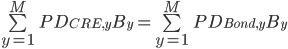
Where:

• is the number of years to maturity
• is the probability of default in year for the CRE loan
• is the probability of default in year for the standard bond
• is the balance outstanding at default in year

Now with this standard PD for the bond defined, we go one step further to define a single average LGD such that the net present value (NPV) of loss on the bond equals the NPV of loss on the CRE loan¹:

i.e.,

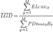
where

• is the expected loss for the CRE loan in year ²
• is the equivalent average LGD

Now that we know we can go one step further to define average equivalent EAD by again equating the expected loss:

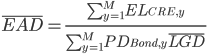
So now for these complex multi-year assets we have the triumvirate of scalar risk statistics required for applications such as Basel capital: PD, LGD and EAD.

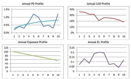
As an illustration, the graphs below show a typical multi-year loss profile for a CRE deal. The probability of default rises and falls with events such as lease expirations and risk. The PD graph also shows the smooth profile of the closest bond. The LGD generally falls over time as amortization and with inflation improve the LTV, but with occasional bumps depending on the cause of default and its correlation with collateral values. For this example the equivalent one-year statistics come out to be PD: 0.29%, LGD: 26%, EAD: $74.

Note that although this LGD has the nice property of equating the expected loss, it is not strictly directly comparable with historical loss given default data. The more accurate comparison is to look at the LGDs per year which are calculated by dividing by . Even more directly, if you are using a simulation method, take the scenario by scenario loss dividend by balance outstanding and compare those results with the historical data.

Dr. Chris Marrison
CEO, Risk Integrated