Publications

This paper deals with the interaction of net operating income, debt servicing, collateral value, reserve accounts, the borrower's worth and the borrower's reputation and how those factors determine the willingness and ability to avoid default. This integrated analysis brings structure to long-standing debates as to the relative importance of the transaction vs. the borrower. The paper gives a structural model for thinking about when a CRE borrower will default and the factors affecting that decision. This framework has implications for both risk assessment and for the structuring of new deals.

Unlike standard retail and corporate loans, commercial real estate (CRE) loans have a significant amount of structure. The decision to default is often modeled as a function of the Loan to Value (LTV) and the Debt Service Coverage Ratio (DSCR). Together these factors are taken as the main predictors with some 'fuzziness' as to whether a particular loan will default for any given combination of LTV and DSCR. This paper pulls apart the borrower's motives and options when facing default, and by looking at the structure of the default decision, it removes much of the 'fuzziness' and gives a clearer picture of the drivers of default.

Each time a payment is due to the lender, the borrower has two options: Option 1 is to make the payment and Option 2 is to not make the payment. If Option 1 is exercised, the borrower will lose the payment amount, but keep the rights to the property. If Option 2 is exercised the borrower will face default costs and may ultimately lose the property.

If the net operating income (NOI) from the property plus its liquid accounts¹ is greater than the debt installment due, then the borrower will exercise Option 1 and make the debt service payment². If the NOI plus accounts are less than the installment, the borrower would have to use funds from other sources to make the payment. In those circumstances the borrower must be both willing and able to pay those additional funds. Let us first look at the borrower's willingness to pay.

Willing to Pay?

If the borrower finds additional funds and exercises Option 1 to pay, the borrower will lose those funds, retain the future revenue and value from the property and continue to be liable for the remaining loan amount. This can be formulated as follows:

Option 1:

Pay:
Receive³:

Net:

Where:

• is the mortgage payment over the decision horizon
• is the net income from the property over the decision horizon
• is the value of liquid assets bound within the deal, e.g., reserve accounts
• is the property value at the decision horizon
• is the normal transaction cost for selling the property⁴
• is the current debt outstanding
• is the principle paid as part of the mortgage payments over the decision horizon

If the borrower exercises Option 2 and does not pay he will save M, but lose the property, lose any reserve accounts, lose his 'reputation⁵', and potentially lose additional money if he has given guarantees:

Option 2:

Pay:
Receive:

Net:

Where:

• is the value of 'reputation' to the borrower
• is the wealth that the bank would be able to access under a personal guarantee (if there is no guarantee, is zero)
• is the transaction cost in a foreclosure

A borrower should be willing to pay if the net outcome of Option 1 is expected to be greater than the net outcome of Option 2, i.e., the rule is pay if:

i.e., if:

The term can be characterized as the expected shortfall in NOI relative to the debt service required. The expected shortfall is a complex function of expected future lease income and operating costs. When using an approach such as cashflow simulation the expected shortfall can be evaluated directly, but for more simple approaches and for illustration in this paper, the expected shortfall can be recast in terms of the average DSCR over the decision horizon. For our purposes the decision horizon is the time when the NOI is expected to recover sufficiently to pay the debt⁶.

To recast in terms of DSCR and LTV, define variables as ratios of debt and debt service:

Where:

• is the number of years to the decision horizon

Divide by to get:

Therefore a borrower should be willing to pay if:

Able to Pay?

Having addressed the borrower's willingness to pay, we now need to look at his ability. One source of external funds is his current liquid wealth⁷ which is comprised of his liquid personal assets, retained earnings from the property, and any loans he can get against his illiquid assets, e.g., second mortgages on his homes or other properties. Estimation of this value can be based on his personal financial statements (if available) with e.g., an 80% multiplier on their liquid assets and a 40% multiplier on their illiquid assets. Properly, the estimated wealth should be conditional on the default event, i.e., what is their wealth in a situation where there is a low DSCR.

Other than their wealth, the other source of funds is his ability to raise cash using the subject property as collateral, e.g., by refinancing the property, getting a second loan or getting a second investor to buy part of the equity. This source depends mostly on the property's LTV. This can be modelled by considering that an investor would be willing to provide funds (or ultimately buy the building), if they were confident that they would be paid back, and that confidence is reflected in discounting factors on the value and NOI. An external investor can be confident of being paid back if:

Where:

• is a haircut on the value⁸
• is a haircut on the NOI
• is the normal, undistressed, cost of selling a property

Dividing by gives:

If the cashflow is completely discounted (, ), the refinancing rule is simply a function of the LTV, i.e., provide funds if:

or,

Willing and Able

Let's now put together the willingness to pay and ability to pay in a numerical example. For the base case let us assume the following:

Remaining amortization 20 years
Interest Rate 6%
Principle payment () 2.7% of debt
Mortgage payment () 8.7% of debt
Expected duration of shortfall () 1 year
Value of reputation () 5% of debt
Cash accessible via personal guarantee () 5% of debt
Cost of foreclosure () 12% of debt
Liquid funds available () 5% of debt
Reserve account () 0% of debt
Factor on value for a third party () 75%
Factor on NOI for a third party () 75%
Cost of un-distressed sale 8% of debt

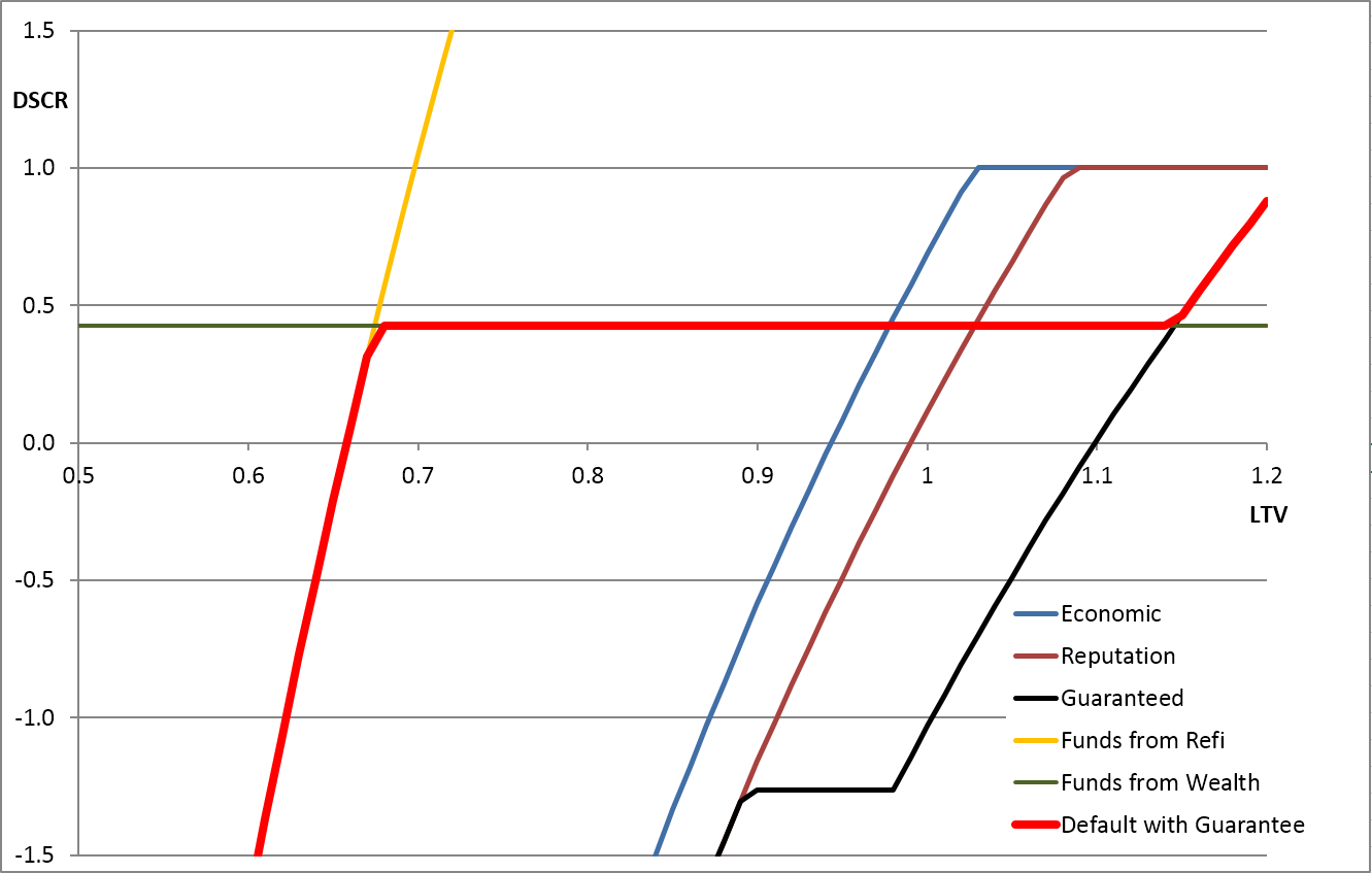
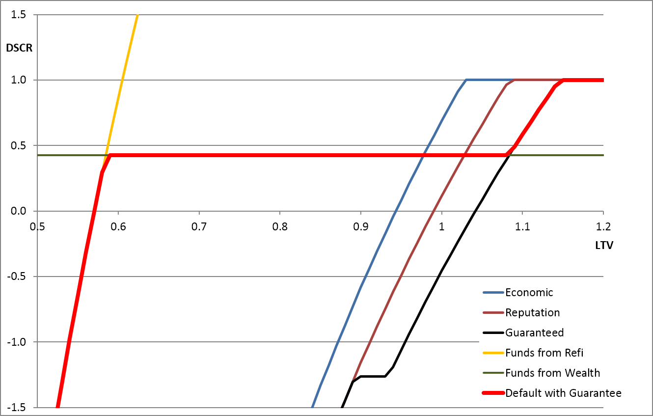
The indifference curves across the LTV/DSCR space for this base-case are shown in the following graph. The blue, brown and black lines show the combinations of DSCR and LTV at which the borrower would be indifferent as to whether they defaulted. To the right of each line the LTV is so poor that the borrower would be willing to give the property to the bank. To the left of each line the borrower would be willing to pay to keep the property.

Default Indifference Curves across the LTV/DSCR space

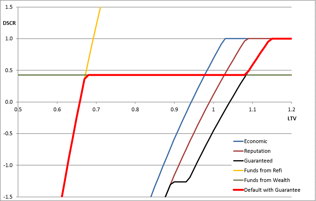
Specifically, the meaning of each line is as follows:

• The blue line assumes there is no guarantee () and no value to reputation () and could therefore be considered the indifference line for willing an 'economic' default.
• The brown line assumes that the value of reputation () is 5% of debt, and therefore the borrower is willing to maintain the loan at worse levels of LTV, i.e., the line moves right.
• The black line assumes that in addition to valuing reputation, the customer has given a guarantee and expects to pay up to 5% of the debt outstanding after a default. This pushes the willingness line further right. However, for better levels of LTV, the guarantee makes no difference because the property value is sufficient to pay off the debt without calling on the guarantee, so the black and brown lines converge for lower LTVs.
• The green line represents the liquid funds () that the borrower has available and therefore represents their ability to pay any shortfall from their own funds.
• The yellow line shows the LTV/DSCR combination at which another investor or bank would be interested in providing funds, thereby making the borrower able to make payments to avoid foreclosure.
• The red line is the combination of the customer being both willing and able to make payments and therefore defines the boundary for default.

Simplistically, the results in this base-case show:

• Below 70% the loan is saved by refinancing.
• Between 70% and 90% LTV it is the borrower's ability to pay that is important, because they are always willing to pay.
• Above 95% LTV, the borrower is unwilling to pay if only economics are important (e.g., in a CMBS), but the cost of reputation and personal guarantees (e.g., for bank customers) can stretch the willingness up to 105% or 115% LTV.

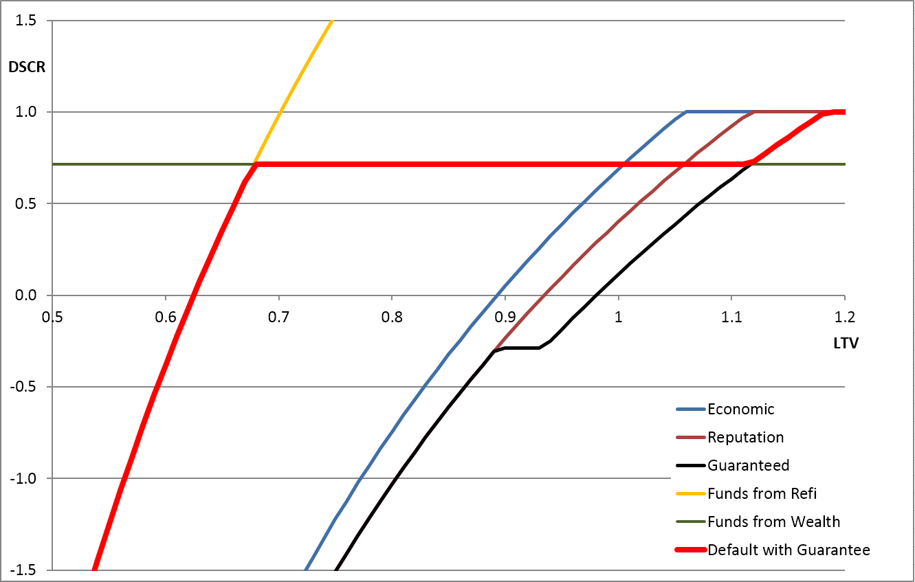
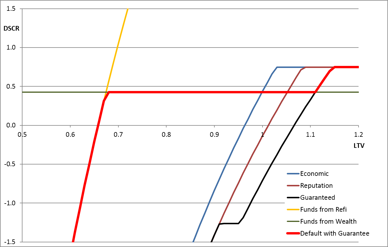
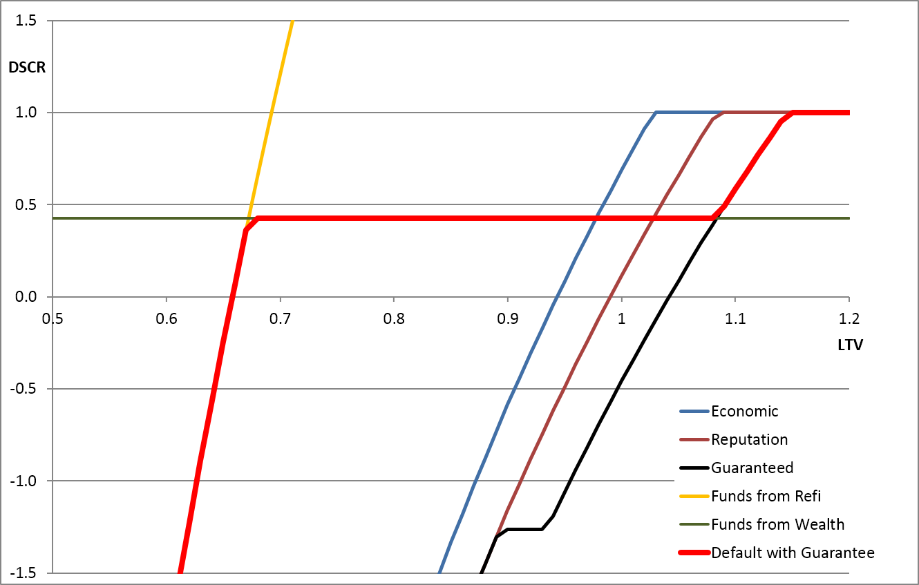
Sensitivity to Parameter Values

Clearly many of these parameters are difficult to quantify for individual borrowers and situations, but most of the parameters are implicitly valued by lending and credit officers in making their decisions. Some factors such as the accessible wealth () can be based on evidence like personal financial statements, other factors such as the decision horizon () can be estimated by simulating market conditions and projecting the future possibilities for NOI.

The charts below show the effect of varying individual parameters. Each graph shows the effect of varying one parameter. The key result in each case is the red default-line. The most important movement of the line is caused by changes in the borrower's ability to pay from their own funds () relative to the expected length of time () that the shortfall is expected to occur. The other factors certainly make a difference to the results, but the structure of the model is reasonably robust and the other parameters would need to be shifted to unreasonable levels to make a large difference to the form of the results.

Base-case

Reputation Value () 5% to 10%

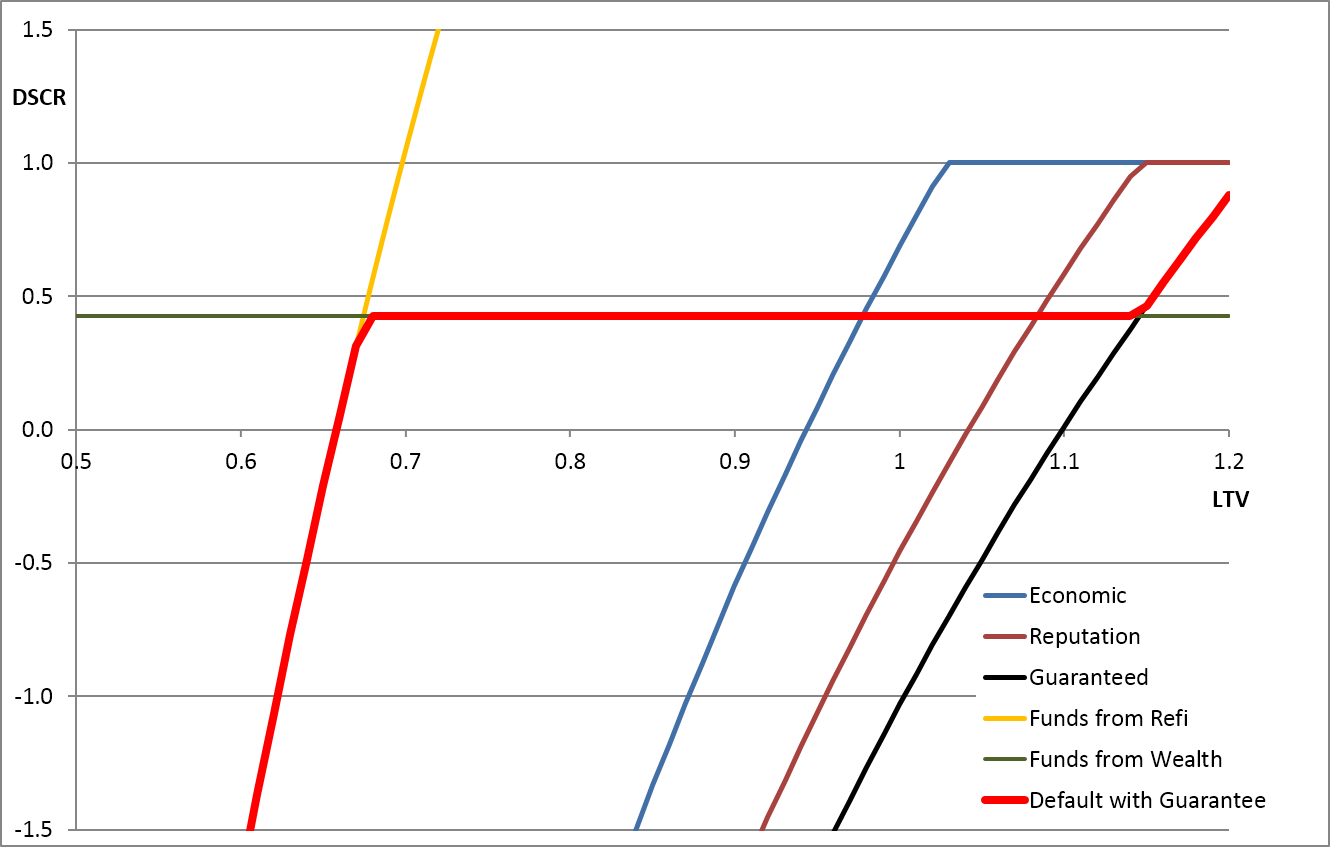
Personal Guarantee () 5% to 10%

Liquid Funds () 5% to 10%

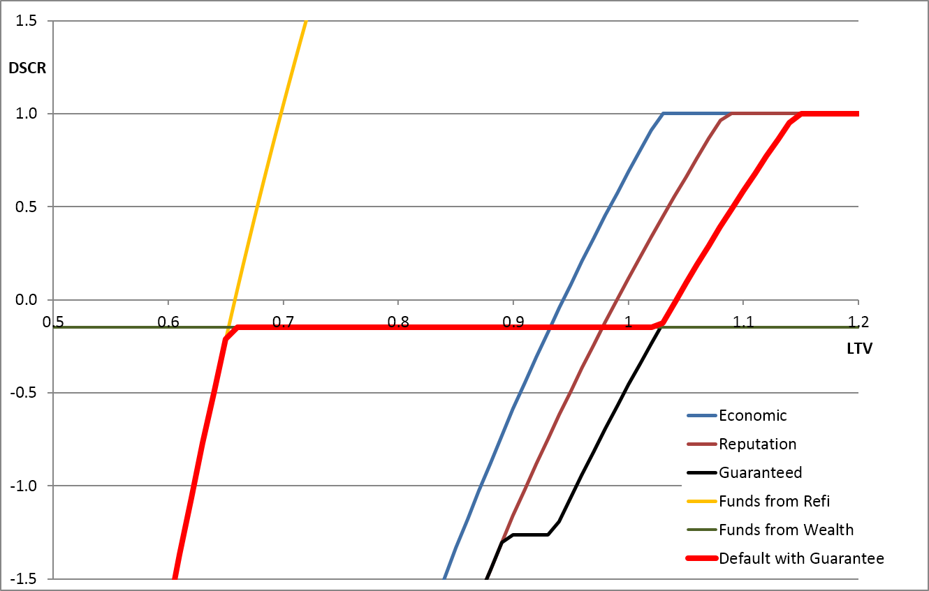
Decision Horizon () 1 year to 2 years

Reserve Account () 0% to 2.2% (3 months)

Value Factor () 75% to 65%

Cashflow Factor () 75% to 65%

Conclusions

It is important to note that although the bulk of the paper discusses the default logic in terms of DSCR with parameters as a percentage of debt, this is only for illustration to show the results in familiar terms. More fundamentally the default logic is given by the original equation, i.e., a borrower should be willing to pay if:

In each circumstance these elements may be evaluated in absolute terms to assess the willingness to default. Also note that this default decision is made at the time and situation when a payment is due, rather than, for example, looking at the probability of default based on LTV and DSCR a year previously.

Overall this analysis provides three insights:

• It shows the structure of the problem and the relationship between the key elements to be considered.
• It guides the shape of the default boundary when projected onto the DSCR/LTV plane.
• It shows the credible ranges for default decisions, e.g., under certain circumstances it is perfectly possible for a deal to not default when it has an LTV of 110% and a DSCR of -20% (e.g., with expenses but no income).

Returning to our original point about reducing the fuzziness (or probabilistic uncertainty) around using LTV and DSCR for estimating defaults, what this analysis shows is that some of the fuzziness comes from failing to include factors such as , , and in the analysis, and another source of the fuzziness is that the dimension of DSCR is too simplistic and is a distortion of actual default logic.

The main usefulness of this analysis is to give a single integrated framework for assessing debt servicing, collateral value, reserve accounts, customer's worth, reputation and guarantees.

Dr. Chris Marrison
CEO, Risk Integrated